AI proved a major quantum complexity conjecture. What does it mean?

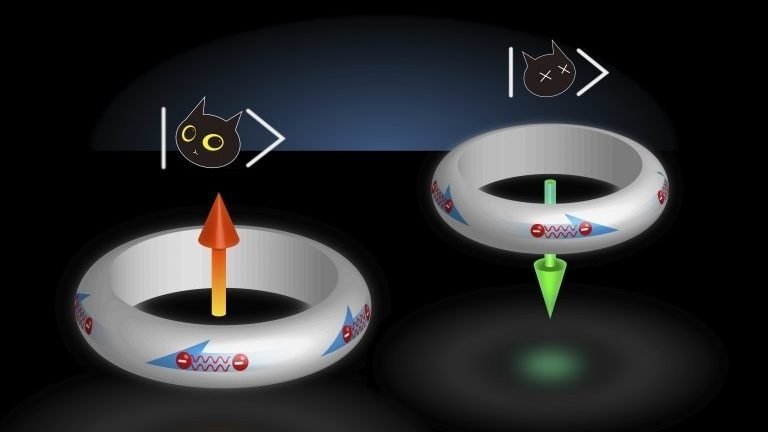
If you work with a normal computer — a classical computer — you’re used to two foundational ideas:

• the idea of bits, where information gets encoded as a “0” or “1” within some sort of storage medium or mechanism,
• and the idea of operations that can be performed on those bits (or “gates” that those bits can be passed through), which represent the possible computations that can be conducted with those bits.

Some problems can be solved very efficiently with classical bits and classical gates, like four-function (+, -, ×, ÷) mathematics, while other problems can only be solved extremely inefficiently with classical bits and classical gates, with the traveling salesman problem being a legendary example of such a “hard” problem.

If you bring in the additional possibilities associated with a quantum computer, however, you no longer have just classical bits and classical gates, but qubits and fundamentally quantum gates. One of the biggest questions in all of computer science is this: which questions and problems, and under which conditions, will the additional options provided by these qubits and quantum gates result in a major computational speedup, and by how much?

That speedup is known as either quantum supremacy or quantum advantage. Which useful problems will experience a quantum advantage, and by how much? That’s one of the main goals of the field of quantum complexity. One of the central open problems in that field, the Aaronson-Ambainis conjecture, has just been solved: by an AI company. Here’s what it does — and doesn’t — mean.

Many of the different computational complexity classes of problems are shown. The innermost spaces require the smallest amounts of writeable memory in order to solve them, while the larger spaces require larger amounts of writeable memory in order to solve them. Examples, from innermore to outermore complexity classes, include problems that can be solved in logarithmic time, polynomial time, nondeterministic polynomial time, and exponential time, among others.

What you see, above, is a map of what’s known as different complexity classes in computer science. Any computational problem is one where you can identify a problem, write down an algorithm for solving that problem, computationally execute that step-by-step algorithm for the specific input associated with that problem, and get an answer. That answer can be a simple binary (yes/no; true/false) answer, which comes for problems that are decision-type problems. However, computational problems include ones that require a more complex quantitative answer: a function problem, a counting problem, or an optimization problem (such as the traveling salesman problem) are all examples of problems more complex than decision problems.

One of the most important complexity classes is known as P. P contains all of the problems that can be solved in polynomial time: generally regarded as “efficiently solvable” problems. If you have a deterministic Turing machine, you can solve a problem of class P using a polynomial amount of computational time. If you’ve ever heard of the famed P versus NP conjecture, it’s a debate over whether problems that are “NP hard,” or which seem to require a nondeterministic amount of polynomial time to solve, could actually ever be solved in polynomial time. It is one of the unclaimed Millennium Prize Problems.

The difficulty of factoring semiprimes, or large integers in general, forms the basis of RSA public-key cryptography. If someone has the key, i.e., one of the prime factors, it becomes computationally easy and fast to factor it. However, if you don’t have the key, it’s very computationally expensive, as large-scale fault-tolerant computers that can implement Shor’s algorithm are not yet available.

Here’s an example that might help you understand the difference between P and NP: I’m going to give you a number, and we’re going to ask if this number is prime. As a simple example (yes, your computer can do this easily), we’re going to pick a relatively small number: 70,747. Is it prime? If we wanted to write an algorithm to determine whether it was prime, you can imagine:

• dividing by 2,
• dividing by 3,
• dividing by 5,
• dividing by 7,
• dividing by 11,
• dividing by 13,
• dividing by 17,

and so on and so on, until you found a prime number that it was divisible by. Either you’d eventually find one, and so you’d know it wasn’t prime, or you would get to a number that was bigger than the square root of the number without finding one, and that would tell you it was prime.

For the number I gave you, 70,747, this algorithm would eventually find that it’s divisible by 263, and that when you divide 70,747 by 263, you find that its other divisor is 269. Finding out if 70,747 is a prime number is an example of an NP problem, but if I give you either 263 or 269, verifying that it’s not prime is easy: an example of a P problem. For much larger numbers — like 80-digit numbers, for example — the verification is easy if you know the counterexample, but demonstrating that an “actually prime” 80-digit number is prime is incredibly computationally difficult. It’s not something that, with today’s computational technology, we can easily or readily do.

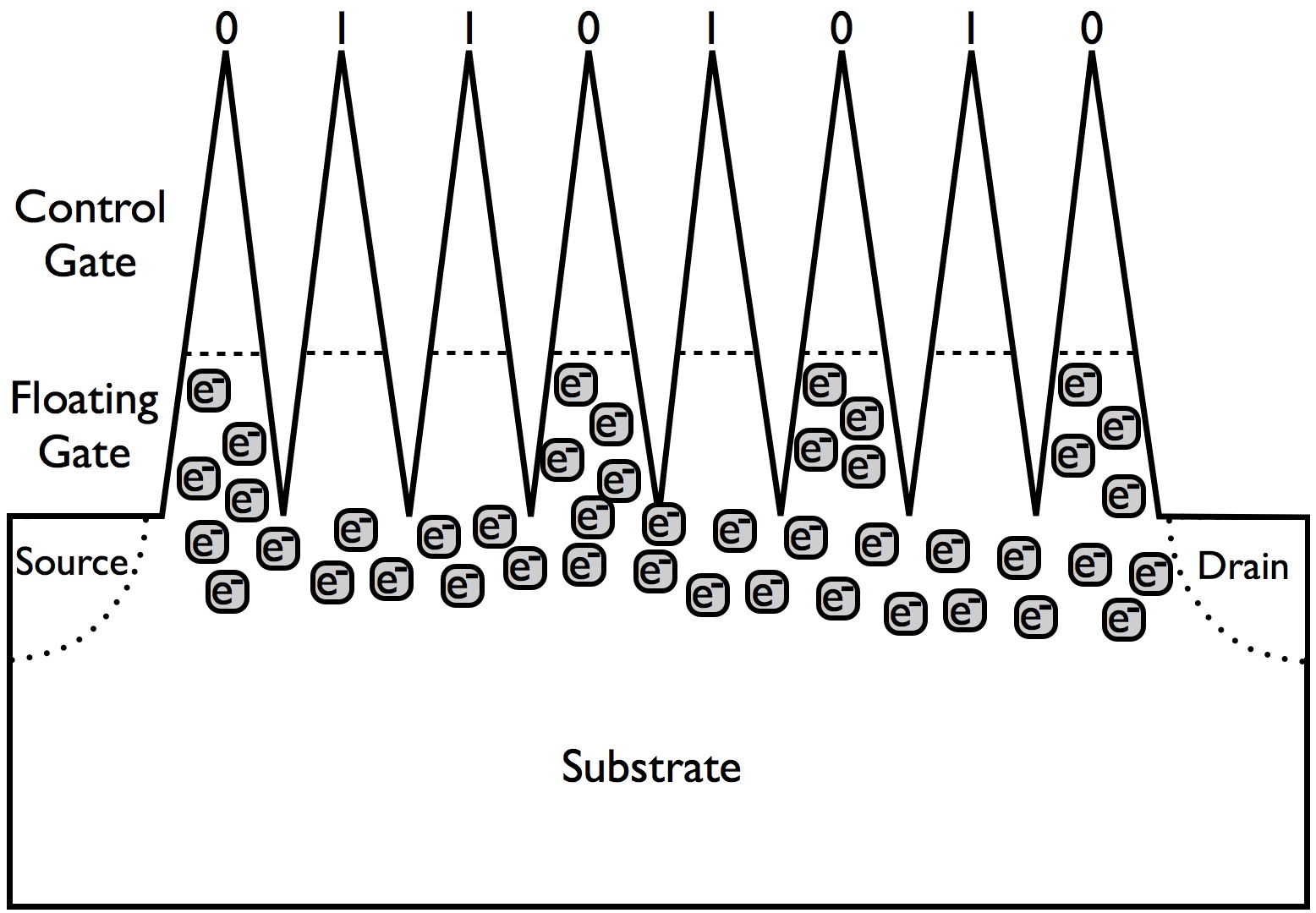
The way solid-state storage devices work today is by the presence or absence of charged particles across a substrate/gate, which inhibits or allows the flow of current, thereby encoding a 0 or a 1. In principle, we can move from bits to qubits by having, instead of a gate with a permanent charge, a quantum bit that reads out only either a 0 or 1 when measured, but that can exist in a superposition of states while operations are being performed on it.

Now that we know what different computational complexity classes are, we can turn to the other aspect to this problem: the difference between classical and quantum computers, and the hope of a “quantum speedup” for certain classes of problems. While classical computers are limited to bits and standard classical operations — operations such as AND, NOT, and OR — quantum computers have inherently quantum versions of both of these in addition to just the classical versions of what’s available.

The first major difference is that instead of just bits, which are always in a state that’s a “0” or a “1” with zero exceptions, qubits can also exist in an intermediate state. That intermediate state can be a superposition of “part 0” and “part 1” that isn’t necessarily either 100%/0%, 50%/50%, or 0%/100%, but any value in between them. As long as it sums up to 100% probability at every moment in time, all states are allowed. The amount of “0” and the amount of “1” that it has changes for three reasons:

• as a result of operations performed on it,
• as a result of a measurement of the state (which always collapses it to either a “0” or a “1”),
• or as a result of time-evolution.

Of course, since this quantum computer isn’t a perfectly isolated environment, there are also sources of noise and errors from the surrounding particles in the system. Therefore, there are also errors introduced, so that the fidelity of your quantum computer is never perfect. Regardless, the fundamental principle holds: qubits can be a mix of “0” and “1” states combined.

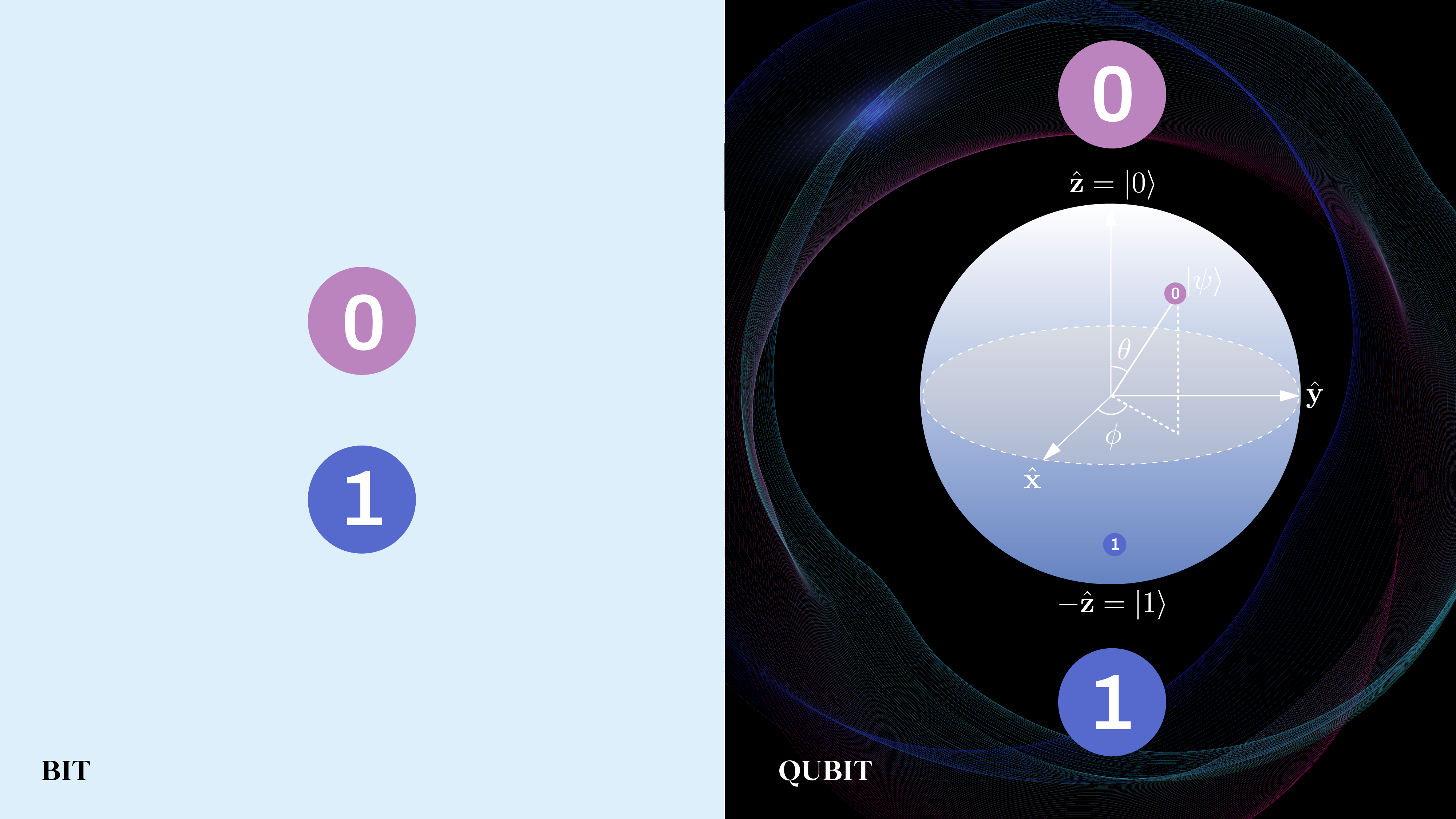
On the left, a classical “bit” is illustrated: a two-state system that can have either “0” or “1” as its value. On the right, a quantum two-state system, or qubit, is shown. When you make a measurement, you’ll always observe either a “0” or a “1” in practice, but when you perform operations on that qubit, you act on the indeterminate state represented by the arrow shown on the sphere. In quantum physics, there is no way to predict what the quantum state of an indeterminate state, composite state, or superposition of states is going to be ahead of time; you can only predict a statistical spectrum of outcomes probabilistically, with the act of measurement required to reveal its physical properties at any moment.

There are also inherently quantum gates: gates that don’t just transform bits from their current state to the opposite state or allow them to remain the same, but rather can transform the qubit from any initial state to any final state in a way that conserves total probability. This can take on many forms.

• There are Pauli gates, which are single-qubit gates that can perform bit-flips, phase-flips, or combinations of the two.
• There are Hadamard gates, which are single-qubit gates that transform an initially pure state (a “0” or a “1”) into a mixed state that’s an equal superposition of both options.
• There are CNOT gates, which are multi-qubit gates that use both a control qubit and a target qubit, flipping the target qubit depending on the state of the control qubit.

And there are many other gates as well that are inherently only available to quantum computers.

However, it’s important to recognize that you can always use a number of classical gates and operations in order to reproduce, simulate, or “hold enough information” to approximate any qubits and quantum gates to whatever level of precision you desire. While you might think that an inherently quantum system would require a quantum computer, with qubits and quantum gates, to model it, it’s been known for many decades that is not the case: the Church-Turing thesis dictates that any computable function can indeed be in-principle computed by a classical computer. There is no problem that absolutely requires a quantum computer in order to solve it.

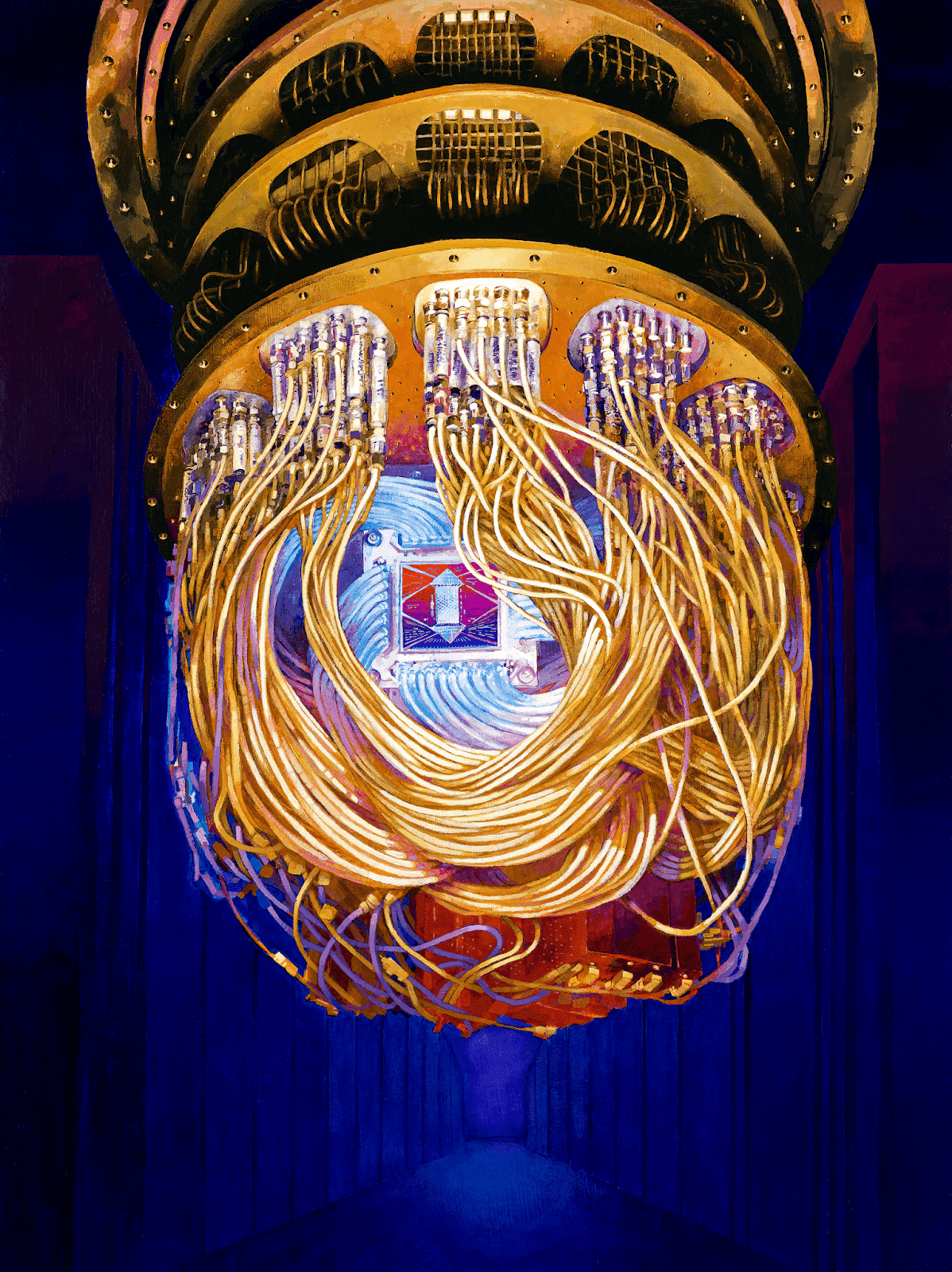
This rendition of a Sycamore processor mounted in a superconducting cryostat illustrates how Google’s quantum computer looked prior to the release of its Willow chip. Although qubits offer some computational advantage over classical computers, there is nothing that can be fundamentally simulated on a quantum computer that can’t also be simulated on a classical one. The goal of quantum computing is to achieve quantum advantage: quantum supremacy for a useful, practical problem.

But the Church-Turing thesis says nothing about the efficiency of that computability. There are some problems that might be extremely inefficient to solve on a classical computer but extremely efficient to solve on a quantum computer; it’s expected that physical quantum mechanical problems, like simulating the double-slit experiment, fall into this category. However, for a wide variety of problems, it’s unclear how much of a speedup a quantum computer can get you versus a classical computer.

Furthermore, because it’s so easy to have extraordinarily large numbers of bits — megabits, gigabits, terabits, petabits, etc. — on a classical computer, but difficult to maintain even a few dozen qubits for more than a tiny fraction of a second of coherence, even in cases where it’s possible to gain a quantum advantage, it’s incredibly difficult to gain a practical quantum advantage.

How complex is a computational problem, anyway? And what’s the difference between the complexity of a classically-stated problem versus the complexity of a quantum-stated problem? That’s where the idea of quantum computational complexity comes in, and if we want to understand what the latest advance of proving the Aaronson-Ambainis conjecture is, that’s where we need to go.

This graph shows whether problems are useful/not useful (x-axis) versus how difficult they are for classical computers to solve (y-axis). While random circuit sampling is the most difficult known task for a classical computer to achieve, it is also arguably the most useless application a quantum computer can be tasked with.

We’ve already talked about the P complexity class of problems: problems that can be solved in deterministic polynomial time. There’s a more general class of problems that includes, but isn’t restricted to, deterministic problems: probabilistic problems. If you can write an algorithm for a problem where the computer can:

• flip coins and make random decisions,
• runs in polynomial time,
• and each time you run the algorithm, gives the wrong answer to a “yes/no” question no more than one-third of the time,

you fall into the class known as BPP: bounded-error probabilistic polynomial time problems. One step up from BPP, which is to say it includes BPP but is even more general, is BQP: an algorithm that can be run on a quantum computer instead of just on a classical one.

According to Scott Aaronson, the “Aaronson” in the Aaronson-Ambainis conjecture, attempting to separate P from BQP is where the whole idea of the conjecture came from. If you imagine having a quantum algorithm making a certain number of queries to an input string, is it possible to make a purely classical simulation that made a polynomially-scaled number of queries to that same input string, and that approximates the quantum algorithm’s success for most values of that input string? If you could, you’d demonstrate that you don’t get (very much of a) quantum advantage from using a quantum algorithm for this class of problems.

This illustration shows containments of various randomized complexity classes within the domain of PSPACE. P is a subset of ZPP, which is within the intersection of RP and coRP, which are both contained entirely within the larger class of BPP, which is itself contained within BQP, PP, and PSPACE, ascendantly.

As Aaronson puts it, “It would underscore that superpolynomial quantum speedups depend on structure.” Although that specific problem was never solved by anyone, it led Aaronson, in 2008, to notice that a solution would follow from a conjecture about influences in lower-degree polynomials. Then, in 2011, Andris Ambainis was working on a related problem about whether there was a polynomial relation between randomized and quantum querying simulations for partial functions with permutation symmetries. Aaronson and Ambainis worked together to put out a now-15-year-old paper called The Need for Structure in Quantum Speedups.

Thinking back to the problem of factoring large numbers (or determining if they’re prime), a quantum computer can only “defeat” the classical computer if it needs to query the initial input number exponentially fewer times than the classical computer does. If it’s only “polynomially” fewer times, you won’t get the necessary speedup for quantum advantage. The Aaronson-Ambainis conjecture states that if you want to determine that you don’t get the necessary speedup, it is sufficient to show that the ordinary computer can imitate the quantum computer with only a polynomial-time number of additional queries. It still takes more queries, but only “a few” more queries, so there’s no quantum advantage there.

Although many claim that the advent of quantum computing will lead to a speed-up in computations across-the-board as compared to classical computers, this is wildly unlikely to be the case. Instead, the best computers will be hybrids: capable of leveraging the quantum portion for applications where quantum advantage can be achieved, but resorting to classical computing techniques for all other (i.e., most) applications.

But was the conjecture true? It was proven true for certain special cases, and it was very recently proven (in August of 2026) that if your quantum algorithm looks at your input in a fixed number of parallel rounds, you also don’t get exponential speedups. While the AI-generated proof certainly built upon this already-substantial amount of earlier work, the authors of that August 2026 paper wrote,

“This is a huge result. It resolves a decades-old conjecture with important implications for the nature of problems that admit quantum speedups. The proof draws on and extends several lines of work in the analysis of Boolean functions and probabilistic combinatorics. Everything is brought together in a rather magical way.”

What has been a longstanding conjecture — a conjecture that was widely thought to be true — has now been proven. The impact on practical quantum computing, however, is zero. It was already generally thought that you’d need some kind of special structure to get a significant speedup from a quantum computer over a classical computer, and this has now been proven to indeed be the case. In quantum physics, quantum chemistry, and materials science, we still expect that speedup to genuinely be present.

The now-proven Aaronson-Ambainis conjecture concerns the average change in a polynomial’s value when a bit is flipped from 0 to 1 or back from 1 to 0. The number of switches is related to the polynomial’s degree, and the proof of the conjecture shows that you do not get an exponential speedup from using a quantum computer over a classical computer from this set of procedures.

Quite fortuitously, Scott Aaronson actually gave his own take on the proof, and he’s quite impressed. However, as he noted:

• the proof of the Aaronson-Ambainis conjecture doesn’t kill quantum supremacy,
• it doesn’t change how we’re going to build quantum computers,
• it doesn’t mean that Scott himself actually understands the proof as it was presented (he notes that he’s no longer an expert on his own conjecture),
• it only rules out a class of quantum speedups that most people didn’t think would exist,
• and that right now is an age where a large number of longstanding open problems in all of computer science and mathematics are falling, so it’s no surprise that this conjecture has now been proven.

The only type of quantum supremacy that’s dead is a type that would have meant quantum querying yes-or-no problems relative to random oracles, which was long conjectured to not exist anyways. No form of quantum supremacy that is actually conjectured to exist is affected by this proof!

So it’s great that we’ve proven and confirmed an expected-to-be-true conjecture, and it’s great that people with expertise are impressed at the proof itself. If we hope for quantum advantage, it’s useful to know where we should and shouldn’t be looking, and this tells us one place, for certain, where we definitely shouldn’t be looking any further. Still, all of the math and computer science (and physics) proofs that have arrived from AI have heavily built on human-made work that led us up to this point.

It makes one wonder: is AI close to reaching the limits of what it will actually be able to solve? And if the answer is no, will there be any humans around who can even understand what those next-level discoveries will mean? Only time will provide the answer to those questions.